Water Treatment Plant
Categorizing the plant's operation state using sensor data suing SVMs.
This problem comes from the daily measures of sensors in an urban waste water treatment plant. The objective is to classify the operation state of the plant at each of the stages of the treatment process using SVMs and KNN. The plant is constituted by a primary settler, a biological reactor, and a secondary settler. After the biological reactor, where the level of substrate is reduced by the action of microorganisms, the water flows to the secondary settler where the biomass sludge settles. Clean water hence remains at the top of the settler and can be easily carried out of the plant. A portion of the sludge is returned to the bioreactor’s input to maintain an appropriate level of biomass, allowing the oxidation of organic matter, while the rest of the sludge is purged.
Data Documentation
This dataset comes from the daily measures of sensors in a urban waste water treatment plant. The objective is to classify the operational state of the plant in order to predict faults through the state variables of the plant at each of the stages of the treatment process. This domain has been stated as an ill-structured domain.
For more information please read the data documentation.
Attributes
Water treatment plant dataset has 38 attributes. All atrributes are numeric and continuous:
-
Q-E (input flow to plant)
-
ZN-E (input Zinc to plant)
-
PH-E (input pH to plant)
-
DBO-E (input Biological demand of oxygen to plant)
-
DQO-E (input chemical demand of oxygen to plant)
-
SS-E (input suspended solids to plant)
-
SSV-E (input volatile supended solids to plant)
-
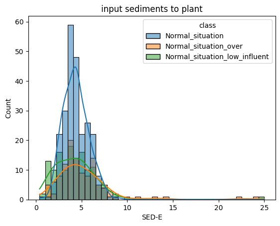
SED-E (input sediments to plant)
-
COND-E (input conductivity to plant)
-
PH-P (input pH to primary settler)
-
DBO-P (input Biological demand of oxygen to primary settler)
-
SS-P (input suspended solids to primary settler)
-
SSV-P (input volatile supended solids to primary settler)
-
SED-P (input sediments to primary settler)
-
COND-P (input conductivity to primary settler)
-
PH-D (input pH to secondary settler)
-
DBO-D (input Biological demand of oxygen to secondary settler)
-
DQO-D (input chemical demand of oxygen to secondary settler)
-
SS-D (input suspended solids to secondary settler)
-
SSV-D (input volatile supended solids to secondary settler)
-
SED-D (input sediments to secondary settler)
-
COND-D (input conductivity to secondary settler)
-
PH-S (output pH)
-
DBO-S (output Biological demand of oxygen)
-
DQO-S (output chemical demand of oxygen)
-
SS-S (output suspended solids)
-
SSV-S (output volatile supended solids)
-
SED-S (output sediments)
-
COND-S (output conductivity)
-
RD-DBO-P (performance input Biological demand of oxygen in primary settler)
-
RD-SS-P (performance input suspended solids to primary settler)
-
RD-SED-P (performance input sediments to primary settler)
-
RD-DBO-S (performance input Biological demand of oxygen to secondary settler)
-
RD-DQO-S (performance input chemical demand of oxygen to secondary settler)
-
RD-DBO-G (global performance input Biological demand of oxygen)
-
RD-DQO-G (global performance input chemical demand of oxygen)
-
RD-SS-G (global performance input suspended solids)
-
RD-SED-G (global performance input sediments)
Code Explanation
Import Libraries
The code begins by importing the necessary libraries, including pandas and numpy. These libraries are used for data manipulation and analysis.
Read Data
The water treatment plant dataset is read from Google Drive using the pd.read_csv() function. The shape of the loaded dataframe is printed.
Display Samples
The top few rows of the dataset are displayed using water_data.head(). This shows how the data looks.
Data Summary
A concise summary of the dataframe is printed using water_data.info(). It provides information about non-null counts and data types for each column.

Data Visualization
- Histograms: Histograms are created using
sns.histplot()to visualize the distribution of features likePH-E,SSV-E, andSED-E. - Bar Plots: Bar plots are used to show relationships between features like
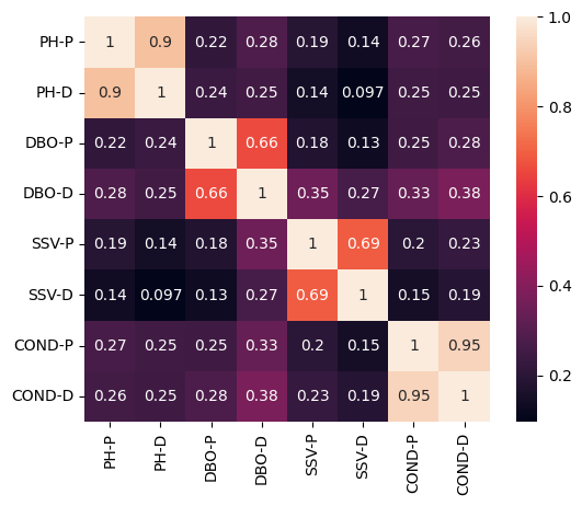
PH-Eand class labels. - Correlation Matrix: A heatmap displays correlations between features extracted from primary and secondary settlers.
- Scatter Plots: Scatter plots show relationships between features like
PH-PandPH-D.

Data Preprocessing
- Missing Value Imputation: The KNNImputer is used to impute missing values in the dataset.
- Feature Normalization: Features are normalized to a range between 0 and 1 using MinMaxScaler.
- Label Encoding: Class labels are transformed into integer values.
Model Training and Evaluation
- Linear SVM: A linear SVM model is trained and evaluated on training and test data.
- Kernel SVM (RBF): A kernel SVM model with an RBF kernel is fine-tuned using GridSearchCV for hyperparameter optimization.
Results
- Linear SVM achieved a training accuracy of approximately 70% and a test accuracy of around 66%.
- Kernel SVM (RBF) with optimized hyperparameters achieved a training accuracy of 98% and a test accuracy of 83%.